Meaningful results for meaningful hypotheses
A tutorial on meaningful hypothesis testing with Bayes factors using ROPEs
Stop asking if an effect is “exactly zero” for experimental designs. It’s not a helpful question. Instead, concentrate on interpreting the actual meaning of the difference between two conditions using Bayesian inference.
How to decide if an effect is meaningful in Bayesian inference?
After years of null hypothesis significance testing (NHST), you might have finally made the switch to Bayesian inference. You set priors, run the models you want to run, and estimate posterior distributions. Great! But what now? When writing up their Bayesian results, people often wonder how to decide whether results are meaningful or not. We have been there ourselves.
Nowadays, more and more researchers move away from NHST toward Bayesian inference (e.g. van der Schoot et al. 2017) and are faced with the same conceptual hurdle because decision procedures are not an inherent part of the Bayesian workflow. There are several approaches to hypothesis testing within the Bayesian framework, of course. Unfortunately, many of them, such as various forms of calculating the Bayes Factor, are either conceptually challenging, computationally (too) costly, or both.
A computationally feasible and intuitive way
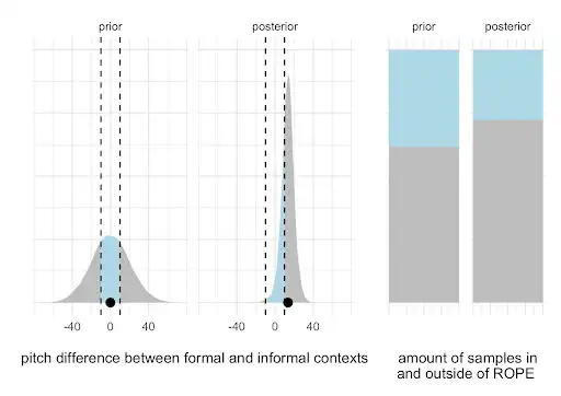
In our new tutorial, we walk you through a lesser known form of Bayes Factor calculation using the Savage-Dickey approximation ( Dickey & Lientz 1970). This form of inference is not only conceptually intuitive and computationally efficient, but it also allows us to tackle another conceptual issue with traditional hypothesis testing: Researchers coming from NHST tend to test whether differences between conditions are smaller or greater than exactly zero (i.e. testing point-0 hypotheses). But not every difference that is not zero is meaningful for either theoretical or practical purposes. In our tutorial, we use a data set on pitch perception by Korean speakers in formal and informal contexts. The researchers want to know if speakers use meaningfully higher or lower pitch in these two social contexts.
To test this hypothesis, we suggest the following workflow:
We define the smallest effect size of interest (SESOI, see Lakens 2017) and implement it as a region of practical equivalence (ROPE, see Kruschke 2018). Defining a SESOI is not easy and requires a good quantitative understanding of the phenomena. In our example, we define the ROPE in terms of the acoustic differences that lead to a certain accuracy performance in a forced-choice perception task (the so-called just-noticeable-difference). The simplified idea is that if you cannot reliably hear a certain acoustic difference, then the difference should not matter for communication.
For the difference between contexts, we quantify the proportion of posterior samples inside of the ROPE (i.e. the posteriors are practically equivalent to 0, indicating no meaningful results) relative to the proportion of posteriors outside of the ROPE (i.e. the posteriors represent meaningful differences). We do this for both the posterior distributions before observing the data (i.e., priors only) and after observing the data (i.e., priors combined with the likelihood).
By comparing these probabilities to each other, we can calculate how the evidence for a meaningful difference shifts when observing the data. This shift is the Bayes Factor, that lets us quantify evidence for and against a meaningful pitch difference between contexts.
The proposed workflow is not new ( Wagenmakers et al. 2010), but unfortunately not widely known across the behavioral sciences. This computationally lightweight decision procedure is conceptually intuitive and encourages us to critically reflect on what it means for an effect to be truly meaningful. Win-win.
Where to start if you are new to Bayesian inference?
Our tutorial is basically a long awaited 2nd sequel (!?) of Bodo Winter’s original introduction to linear mixed effects models from 2013. This tutorial was widely shared and cited because it was one of the first very accessible introductions to linear mixed effects models within NHST. Six years later, we wrote a sequel that used the original example problem and demonstrated how to implement it into a Bayesian workflow. Now, another 6 years later, we thought it was time to drop Part 3, sticking to the same phenomenon and data set as the original, finally bringing the trilogy to a “meaningful” conclusion.
Contact information
Email: timo.roettger@iln.uio.no
Bluesky: @timoroettger.bsky.social
LinkedIn: linkedin.com/in/timo-b-roettger/
Website: timo-b-roettger.github.io

Email: mchfranke@gmail.com
Bluesky: @meanwhileina.bsky.social
Website: michael-franke.github.io/heimseite/
